Special Topics in Complexity Theory, Fall 2017. Instructor: Emanuele Viola
1 Lecture 1, Scribe: Chin Ho Lee
In this first lecture we begin with some background on pseudorandomness and then we move on to the study of bounded independence, presenting in particular constructions and lower bounds.
1.1 Background
Let us first give some background on randomness. There are 3 different theories:
(1) Classical probability theory. For example, if we toss a coin 
![\Pr [010101010101] = \Pr [011011100011]](https://s0.wp.com/latex.php?latex=%5CPr+%5B010101010101%5D+%3D+%5CPr+%5B011011100011%5D&bg=ffffff&fg=333333&s=0&c=20201002)
(2) Kolmogorov complexity. Here the randomness is measured by the length of the shortest program outputting a string. In the previous example, the program for the second outcome could be “print 011011100011”, whereas the program for the first outcome can be “print 01 six times”, which is shorter than the first program.
(3) Pseudorandomness. This is similar to resource-bounded Kolmogorov complexity. Here random means the distribution “looks random” to “efficient observers.”
Let us now make the above intuition precise.
Definition 1.[Pseudorandom generator (PRG)] A function 


(1) the output of the generator must be longer than its input, i.e., 
(2) it should fool 

![\Pr [t(U_n) = 1] = \Pr [t(f(U_s)) = 1] \pm \epsilon](https://s0.wp.com/latex.php?latex=%5CPr+%5Bt%28U_n%29+%3D+1%5D+%3D+%5CPr+%5Bt%28f%28U_s%29%29+%3D+1%5D+%5Cpm+%5Cepsilon+&bg=ffffff&fg=333333&s=0&c=20201002)
(3) the generator must be efficient.
To get a sense of the definition, note that a PRG is easy to obtain if we drop any one of the above 3 conditions. Dropping condition (1), then we can define our PRG as 

Claim 2. For every class of tests 
Before proving the claim, consider the example where 


We now prove the claim using the probabilistic method.
Proof. Consider picking 
![\begin{aligned} \Pr _f[ | \Pr _{U_s} [ t(f(U_s)) = 1] - \Pr _{U_n}[ t(U_n) = 1] | \ge \epsilon ] \le 2^{-\Omega (\epsilon ^2 2^s)} < 1 / |T|, \end{aligned}](https://s0.wp.com/latex.php?latex=%5Cbegin%7Baligned%7D+%5CPr+_f%5B+%7C+%5CPr+_%7BU_s%7D+%5B+t%28f%28U_s%29%29+%3D+1%5D+-+%5CPr+_%7BU_n%7D%5B+t%28U_n%29+%3D+1%5D+%7C+%5Cge+%5Cepsilon+%5D+%5Cle+2%5E%7B-%5COmega+%28%5Cepsilon+%5E2+2%5Es%29%7D+%3C+1+%2F+%7CT%7C%2C+%5Cend%7Baligned%7D&bg=ffffff&fg=333333&s=0&c=20201002)
if 
1.2  -wise independent distribution
A major goal in research in pseudorandomness is to construct PRGs for (1) richer and richer class 
Definition 3.[
We will show that for this class of tests we can actually achieve error 


For 

Here the length of 


Now we prove the correctness of this PRG.
Claim 4. The 
Proof. We need to show that for every 


The case for 

Lemma 5. There exist finite fields of size 


Remark 6. Ideally one would like the dependence on 


One simple example of finite fields are integers modulo
Theorem 7. Let 

(1) elements in 
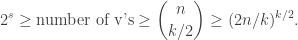
(2) every 
For 
Remark 8. There exist other constructions that are similar to the inner product construction for the case
Note that we can also apply the theorem for larger 
We now prove the theorem.
Proof. Pick a finite field 


(One should think of the outputs of
The analysis of the PRG follows from the following useful fact: For every 
Let us now introduce a terminology for PRGs that fool
Definition 9. We call distributions that look uniform (with error 
We will soon see an example of a distribution where every
1.3 Lower bounds
We have just seen a construction of
Claim 10. For every 


Proof. We use the linear-algebraic method. See the book by Babai–Frankl [1] for more applications of this method.
To begin, we will switch from 


However so far we have not used 

Claim 11. If 
Proof. Suppose they are not and we can write 


Therefore, the rank of
Rearranging gives 
1.4 Who is fooled by -wise independence?
In the coming lectures we will see that 
(1) Suppose we have ![x_1, \ldots , X_n \in [0,1]](https://s0.wp.com/latex.php?latex=x_1%2C+%5Cldots+%2C+X_n+%5Cin+%5B0%2C1%5D&bg=ffffff&fg=333333&s=0&c=20201002)


(2) We will see next time that 
(3)
1.4.1 -wise independence fools AND
We now show that
Claim 12. Every 
Proof. If the AND function is on at most 

![\begin{aligned} \Pr _D[\text {AND on t bits is 1}] \le \Pr _D[\text {AND on k bits is 1}] . \end{aligned}](https://s0.wp.com/latex.php?latex=%5Cbegin%7Baligned%7D+%5CPr+_D%5B%5Ctext+%7BAND+on+t+bits+is+1%7D%5D+%5Cle+%5CPr+_D%5B%5Ctext+%7BAND+on+k+bits+is+1%7D%5D+.+%5Cend%7Baligned%7D&bg=ffffff&fg=333333&s=0&c=20201002)
The right-hand-side is the same under uniform and 
![\begin{aligned} | \Pr _{\text {uniform}}[AND = 1] - \Pr _{\text {k-wise ind.}}[\mathrm {AND} = 1] | \le 2^{-k} . \end{aligned}](https://s0.wp.com/latex.php?latex=%5Cbegin%7Baligned%7D+%7C+%5CPr+_%7B%5Ctext+%7Buniform%7D%7D%5BAND+%3D+1%5D+-+%5CPr+_%7B%5Ctext+%7Bk-wise+ind.%7D%7D%5B%5Cmathrm+%7BAND%7D+%3D+1%5D+%7C+%5Cle+2%5E%7B-k%7D+.+%5Cend%7Baligned%7D&bg=ffffff&fg=333333&s=0&c=20201002)
Instead of working over bits, let us now consider what happens over a general domain 


This is similar to the previous example, except now that the variables are independent but not necessarily uniform. Nevertheless, we can show that a similar bound of 
Theorem 13.[[2]] Let 
![\begin{aligned} \Pr [ \prod _{i = 1}^n X_i = 1 ] = \prod _{i = 1}^n \Pr [X_i = 1] \pm 2^{-\Omega (k)} . \end{aligned}](https://s0.wp.com/latex.php?latex=%5Cbegin%7Baligned%7D+%5CPr+%5B+%5Cprod+_%7Bi+%3D+1%7D%5En+X_i+%3D+1+%5D+%3D+%5Cprod+_%7Bi+%3D+1%7D%5En+%5CPr+%5BX_i+%3D+1%5D+%5Cpm+2%5E%7B-%5COmega+%28k%29%7D+.+%5Cend%7Baligned%7D&bg=ffffff&fg=333333&s=0&c=20201002)
This fundamental theorem appeared in the conference version of [2], but was removed in the journal version. One of a few cases where the journal version contains less results than the conference version.
Proof. Since each
![\begin{aligned} \Pr [\prod _{i=1}^n X_i = 1] = \mathbb{E} [ \prod _{i=1}^n X_i ] = \mathbb{E} [ \mathrm {AND}_{i=1}^n X_i ] = \mathbb{E} [ 1 - \mathrm {OR}_{i=1}^n (1 - X_i)]. \end{aligned}](https://s0.wp.com/latex.php?latex=%5Cbegin%7Baligned%7D+%5CPr+%5B%5Cprod+_%7Bi%3D1%7D%5En+X_i+%3D+1%5D+%3D+%5Cmathbb%7BE%7D+%5B+%5Cprod+_%7Bi%3D1%7D%5En+X_i+%5D+%3D+%5Cmathbb%7BE%7D+%5B+%5Cmathrm+%7BAND%7D_%7Bi%3D1%7D%5En+X_i+%5D+%3D+%5Cmathbb%7BE%7D+%5B+1+-+%5Cmathrm+%7BOR%7D_%7Bi%3D1%7D%5En+%281+-+X_i%29%5D.+%5Cend%7Baligned%7D&bg=ffffff&fg=333333&s=0&c=20201002)
If we define the event 

![\Pr [\bigcup _{I=1}^n E_i]](https://s0.wp.com/latex.php?latex=%5CPr+%5B%5Cbigcup+_%7BI%3D1%7D%5En+E_i%5D&bg=ffffff&fg=333333&s=0&c=20201002)
![\begin{aligned} \Pr [\bigcup _{i=1}^n E_i] = \sum _{i=1}^n \Pr [E_i] - \sum _{i \neq j} \Pr [E_i \cap E_j] + \cdots + (-1)^{J + 1} \sum _{S \subseteq [n], |S| = J} \Pr [\bigcap _{i \in S} E_i] + \cdots . \end{aligned}](https://s0.wp.com/latex.php?latex=%5Cbegin%7Baligned%7D+%5CPr+%5B%5Cbigcup+_%7Bi%3D1%7D%5En+E_i%5D+%3D+%5Csum+_%7Bi%3D1%7D%5En+%5CPr+%5BE_i%5D+-+%5Csum+_%7Bi+%5Cneq+j%7D+%5CPr+%5BE_i+%5Ccap+E_j%5D+%2B+%5Ccdots+%2B+%28-1%29%5E%7BJ+%2B+1%7D+%5Csum+_%7BS+%5Csubseteq+%5Bn%5D%2C+%7CS%7C+%3D+J%7D+%5CPr+%5B%5Cbigcap+_%7Bi+%5Cin+S%7D+E_i%5D+%2B+%5Ccdots+.+%5Cend%7Baligned%7D&bg=ffffff&fg=333333&s=0&c=20201002)
we will finish the proof in the next lecture.
References
