Special Topics in Complexity Theory, Fall 2017. Instructor: Emanuele Viola
1 Lecture 19, Guest lecture by Huacheng Yu, Scribe: Matthew Dippel
Guest lecture by Huacheng Yu on dynamic data structure lower bounds, for the 2D range query and 2D range parity problems. Thanks to Huacheng for giving this lecture and for feedback on the write-up.
What is covered.
- Overview of Larsen’s lower bound for 2D range counting.
- Extending these techniques for
for 2D range parity.
2 Problem definitions
Definition 1. 2D range counting
Give a data structure 
- UPDATE: Add a (point, weight) tuple to the set.
- QUERY: Given a query point
, return the sum of weights of points
in the set satisfying
and
.
Definition 2. 2D range parity
Give a data structure
- UPDATE: Add a point to the set.
- QUERY: Given a query point
Both of these definitions extend easily to the 
2.1 Known bounds
All upper bounds assume the RAM model with word size 
Upper bounds: Using range trees, we can create a data structure for 2D range counting, with all update and query operations taking time 
Lower bounds. There are a series of works on lower bounds:
- Fredman, Saks ’89 – 1D range parity requires
.
- Patrascu, Demaine ’04 – 1D range counting requires
.
- Larsen ’12 – 2D range counting requires
.
- Larsen, Weinstein, Yu ’17 – 2D range parity requires
.
This lecture presents the recent result of [Larsen ’12] and [Larsen, Weinstein, Yu ’17]. They both use the same general approach:
- Show that, for an efficient approach to exist, the problem must demonstrate some property.
- Show that the problem doesn’t have that property.
3 Larsen’s technique
All lower bounds are in the cell probe model with word size
We consider a general data structure problem, where we require a structure 


3.1 Chronogram method [FS89]
We divide the updates into 

where 

Let 


 are disjoint.
 Claim 2. There exists an epoch 

Claim 2 implies that there is an epoch
Idea. : The set 


3.2 Communication game
Having set up the framework for how to analyze the data structure, we now introduce a communication game where two parties attempt to solve an identical problem. We will show that, an efficient data structure implies an efficient solution to this communication game. If the message is smaller than the entropy of the updates of epoch
The game. The game consists of two players, Alice and Bob, who must jointly compute a single query after a series of updates. The model is as follows:
- Alice has all of the update epochs
. She also has an index
- Bob has all update epochs EXCEPT for
- Communication can only occur in a single direction, from Alice to Bob.
- We assume some fixed input distribution
.
- They win this game if Bob successfully computes the correct answer for the query
Then we will show the following generic theorem, relating this communication game to data structures for the corresponding problem:
Theorem 3. If there is a data structure with update time 


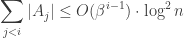
Before we prove the theorem, we consider specific parameters for our problem. If we pick
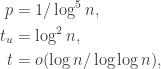
then, after plugging in the parameters, the communication cost is 


Proof.
We assume we have a data structure
Alice’s steps.
- Simulate
. While doing so, keep track of memory cell accesses and compute
.
- Sample a random subset
, such that
.
- Send
.
We note that in Alice’s Step 3, to send a cell, she sends a tuple holding the cell ID and the cell state before the query was executed. Also note that, she doesn’t distinguish to Bob which cells are in which sets of the union.
Bob’s steps.
- Receive
from Alice.
- Simulate
. Snapshot the current memory state of the data structure as
- Simulate the query algorithm. Every time
, Bob checks if
. If it is, he lets
- Bob returns the result from the query algorithm as his answer.
If the query algorithm does not query any cell in 


4 Extension to 2D Range Parity
The extension to 2D range parity proceeds in nearly identical fashion, with a similar theorem relating data structures to communication games.
Theorem 1. Consider an arbitrary data structure problem where queries have 1-bit outputs. If there exists a data structure having:
- update time
- query time
- Probes

Then there exists a protocol for the communication game with 

then the cost is 
We note that, if we had 


Proof. The communication protocol will be slightly adjusted. We assume an a priori distribution on the updates and queries. Bob will then compute the posterior distribution, based on what he knows and what Alice sends him. He then computes the maximum likelihood answer to the query 

We assume the existence of some public randomness available to both Alice and Bob. Then we adjust the communication protocol as follows:
Alice’s modified steps.
- Alice samples, using the public randomness, a subset of ALL memory cells
, such that each cell is sampled with probability
. Alice sends
to Bob. Since Bob can mimic the sampling, he gains additional information about which cells are and aren’t in
Bob’s modified steps.
- Denote by
the set of memory cells probed by the data structure when Bob simulates the query algorithm. That is,
Define the function ![f(z) : [2^w] \rightarrow \mathbb {R}](https://s0.wp.com/latex.php?latex=f%28z%29+%3A+%5B2%5Ew%5D+%5Crightarrow+%5Cmathbb+%7BR%7D&bg=ffffff&fg=333333&s=0&c=20201002)


![\begin{aligned} f_{C'}(z) &:= (\text {Pr}[\text {ans to q } = 1 | C', S \leftarrow z] - 1/2) * \text {Pr}[S \leftarrow z | C'] \end{aligned}](https://s0.wp.com/latex.php?latex=%5Cbegin%7Baligned%7D+f_%7BC%27%7D%28z%29+%26%3A%3D+%28%5Ctext+%7BPr%7D%5B%5Ctext+%7Bans+to+q+%7D+%3D+1+%7C+C%27%2C+S+%5Cleftarrow+z%5D+-+1%2F2%29+%2A+%5Ctext+%7BPr%7D%5BS+%5Cleftarrow+z+%7C+C%27%5D+%5Cend%7Baligned%7D&bg=ffffff&fg=333333&s=0&c=20201002)
In particular,

![\mathbb {E}_{C'}[\max _z |f(z)|] \geq 1/2 \cdot p^t](https://s0.wp.com/latex.php?latex=%5Cmathbb+%7BE%7D_%7BC%27%7D%5B%5Cmax+_z+%7Cf%28z%29%7C%5D+%5Cgeq+1%2F2+%5Ccdot+p%5Et&bg=ffffff&fg=333333&s=0&c=20201002)
In these statements, the expectation is over everything that Bob knows, and the probabilities are also conditioned on everything that Bob knows. The randomness comes from what he doesn’t know. We also note that when the query probes no cells in 

Finishing the proof requires the following lemma:
Lemma 2. For any 


Note that the sum inside the absolute values is the bias when 
References
